Congratulations to our winners:
This page presents the 2014 MEMOCODE design contest. This year's problem is to find the k-nearest neighbors of a given point from a multidimensional dataset. k-nearest neighbors (k-NN) is frequently used in pattern recognition and machine learning applications to find how a newly observed datapoint relates to previously observed ones. Given a set of vectors in a multidimensional feature space, k-NN finds the k closest vectors to a given input vector. The Mahalanobis distance metric, used in biomedical applications, allows quantification of the distance between two vectors in a way that takes into account the covariance across the dimensions of the feature space.
Below you will find a description of the problem, a functional reference implementation (in C), example datasets, and a tool (written in C) to check the correctness of your solution's output. Go to the download section.
Participants will have one month to develop systems to solve this problem. Two winning teams will be selected based on absolute performance and cost-adjusted performance. Each team delivering a complete and working solution will be invited to prepare a 2-page abstract to be published in the proceedings and to present it during a dedicated poster session at the conference. The winning teams will be invited to contribute a 4-page short paper for presentation in the conference program.
To compute k-nearest neighbors, you are given a set of D-dimensional vectors which we will refer to as the dataset and a set of D-dimensional vectors which we will refer to as the input set. The goal is to find the k closest vectors in the dataset for each vector in the input set (based on a given distance metric). For each vector, you will output the indices of the k nearest neighbors in the dataset and their computed distances.
In pseudocode:
for i = 0 to size of inputset {
for j = 0 to size of dataset {
dist(j) = distance between inputset(i) and dataset(j)
}
find and output k smallest dist(j) and their indices (values of j)
}
The next section explains the concept and computation of the distance metric we will use to compute the distance between two vectors.
This section will motivate and define the Mahalanobis distance metric. We will first consider some examples in two dimensions (i.e., \(D=2\)).
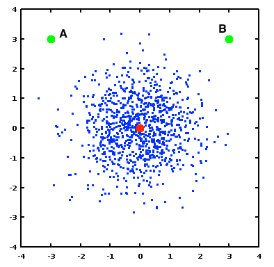
In the following figure, each blue dot represents a (two-dimensional) vector in our dataset, and the red dot (at the origin) represents one particular point from this set. The two green dots (A and B) represent two values from the input set. The goal of this example is to explore how we can quantify the similarity between the red dot and each of A and B, given the characteristics of the dataset.
In this example, the two dimensions of the dataset are not correlated and have equal variance, giving the blue cloud a roughly circular shape. Given this dataset and its distribution, the Euclidean distance between two points provides a good metric for the dissimilarity between them. Thus, we could calculate that the distance from either green point to the red point is $$\sqrt{3^2 + 3^2} = \sqrt{18} = 4.2426,$$ and we can conclude that A and B are “equally similar” to the red point.
However, many datasets exhibit correlation and differing levels of variance amongst their dimensions. For example, we consider the dataset in the following figure.
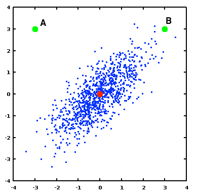
In this new dataset, there is a correlation between the two dimensions (giving the area of blue points a generally diagonal shape), and the variance is not uniform. Each of the green points still has the same Euclidean distance from the red point as in the previous example. However now we can see that in the context of the dataset, B can be considered to be “more similar” to the red point than A is.
The Mahalanobis distance takes this into account by measuring the distance between two points relative to the covariance of the dataset. Let \(S\) represent the covariance matrix of the dataset (or an estimate of it). (For this two-dimensional example, \(S\) is a \(2\times 2\) matrix). The Mahalanobis distance between two points (represented by column vectors \(\vec{x}\) and \(\vec{y}\)) is computed according to $$ \operatorname{dist}(\vec{x},\vec{y}) = \sqrt{(\vec{x}-\vec{y})^T S^{-1}(\vec{x}-\vec{y})}. $$
For this example, $$ S = \left[ \begin{array} 0.96 & 0.69\\ 0.69 & 0.94 \end{array} \right] \quad \text{and} \quad S^{-1} = \left[\begin{array}{rr} 2.20 & -1.61\\ -1.61 & 2.25 \end{array} \right]. $$ So, $$ \operatorname{dist}\left(\left[ \begin{array}{r} -3\\ 3 \end{array} \right], \left[ \begin{array}{r} 0\\ 0 \end{array} \right] \right) = \sqrt{ \left[ \begin{array}{rr} -3 & 3 \end{array} \right] \left[\begin{array}{rr} 2.20 & -1.61\\ -1.61 & 2.25 \end{array} \right] \left[ \begin{array}{r} -3 \\ 3 \end{array} \right] } = 8.315 $$ $$ \operatorname{dist}\left(\left[ \begin{array}{r} 3\\ 3 \end{array} \right], \left[ \begin{array}{r} 0\\ 0 \end{array} \right] \right) = \sqrt{ \left[ \begin{array}{rr} 3 & 3 \end{array} \right] \left[\begin{array}{rr} 2.20 & -1.61\\ -1.61 & 2.25 \end{array} \right] \left[ \begin{array}{r} 3 \\ 3 \end{array} \right] } = 3.318 $$ So, we see that using this distance metric, point B is much closer to the origin than point A is.
To avoid the square root operator (and because the ordering of numbers is preserved under it), your system will use the squared Mahalanobis distance as its cost metric. Given the inverse covariance matrix \(S^{-1}\) you will calculate the distance between D-dimensional vectors \(\vec{x}\) and \(\vec{y}\) as $$ \operatorname{distSq}(\vec{x},\vec{y}) = (\vec{x}-\vec{y})^T S^{-1}(\vec{x}-\vec{y}). $$
Your system will take as input:
For each vector in \(N\), your system will find the \(k=10\) nearest neighbors: the 10 vectors from \(C\) with the lowest distances from the input vector (measured using Mahalanobis distance squared). For each vector in the input set \(N\), your system will output:
The system's input data will be provided in integer form, and all final output distances and indices must be stored as integers. The timed portion of your solution must start with all input data in main system memory, and it must conclude with all output data in main memory.
We have provided a reference software implementation to serve as the functional reference for the contestants' optimized implementations. The reference implementation (kNN.c) reads input files for the dataset \(C\), input set \(N\), and inverse covariance matrix \(S^{-1}\). It then performs the k-NN computation and writes the result indices and distances to output files. For more information on the reference software and its inputs and outputs, please see readme.txt included with the software. Lastly, a Makefile is provided; typing “make runsmall” at the command line will compile the software, run it on a small example dataset, and verify correctness of the results. (Please see below for discussion of the provided datasets and reference solutions.)
Links to the reference code and datasets are available below.
As explained above, the input data are provided in integer form. The range of the input values is limited such that every input element can be represented as a 12-bit two's complement value. As computation progresses, the maximum data values will grow. The provided functional reference software uses the long int (64 bit) datatype, however the full 64 bits are not used. Designers may choose to optimize the datatype as appropriate. A solution will be considered to be correct if its output values match the reference solution with deviations only within the bottom two bits.
Three datasets are provided to aid in validation and development. Each set contains a comparison dataset \(C\), an inverse covariance matrix \(S^{-1}\), and a set of input vectors \(N\). Each set is accompanied by reference solutions, which provide the nearest neighbor and distance results for the problem.
The three datasets provided are named small, medium, and large:
In all cases, \(S^{-1}\) is a \(32\times 32\) matrix, \(D=32\), and \(k=10\).
A program (eval_results.c) to evaluate the correctness of output data is also provided. This program takes in newly-computed output files and the reference solutions and compares them. If there is a discrepancy with the reference solution, the program will compute and report the maximum error.
More information about the dataset input and output file names and instructions for running eval_results are included in readme.txt. Typing “make runsmall” at the command line will compile the reference design, run it on the small example dataset, and verify correctness of the results.
Contestants have one month to implement the system using their choice of platforms such as FPGAs, GPGPUs, etc. The system must be validated using the supplied reference inputs outputs discussed above.
Contest winners will be selected based on the performance of their systems. Performance will be measured based on the “large” dataset or a comparably-sized dataset. The time taken to initialize data and read out the results is excluded from the run time measurement. (See also the comments in reference software's main function.)
As in previous design contests, winners will be chosen in two categories. First, the “pure-performance” award will be based only on the fastest runtime. Second, the “cost-adjusted-performance” award will be chosen by multiplying runtime by cost of the system. For example, a $100 system with runtime of 60 seconds is equivalent to $200 system with runtime of 30 seconds. The cost of the system is based on the lowest listed prices (academic or retail). If no price is available (e.g., using an experimental platform), judges will estimate the system cost. Contestants are encouraged to submit cost estimates of their systems to aid in judging.
Before 11:59:59PM US Eastern Time on July 7, 2014, submit your design solution in a tar or zip file to peter.milder@stonybrook.edu
After your submission you will receive a confirmation email within 24 hours. If you do not receive this information email after 24 hours, please contact peter.milder@stonybrook.edu
Your submission should contain the following items in a single zip or tar file:
Documentation in the form of PowerPoint slides is perfectly acceptable. The quality and conciseness of the documentation will help in judging. The judges will make a best effort to treat the design source files as confidential. The information in other items is considered public.
If you have any questions, please contact Peter Milder.
Peter Milder, peter.milder@stonybrook.edu
This page uses MathJax for displaying mathematical formulas. If your browser has Javascript disabled, formulas will not display correctly.